In the late 1990s, a benchmark problem for computational fluid dynamics (CFD) was published that soon became a standard test for solver accuracy. Known as the “turbulent flow over a backward-facing step,” it simulated a canonical separated flow and was meant to validate that a code could reproduce a well-documented experimental dataset. For years, results from different labs using the same solver agreed within acceptable margins. Then, around 2022, something changed. Groups using the latest version of a popular open-source CFD solver began reporting flow separation lengths that deviated by more than 10% from the benchmark reference. The discrepancy was not random—it was systematic, and it took a painstaking forensic investigation to trace it to a single floating-point threshold that had never been versioned.

A Benchmark That Was Supposed to Be Settled

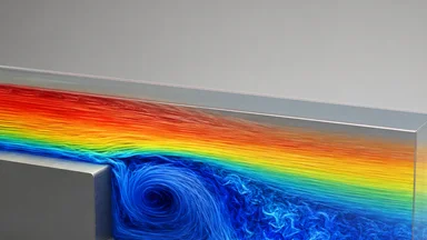
The backward-facing step benchmark, introduced by experimentalists in the 1980s and formalized as a CFD validation case in the 1990s, has been cited in thousands of studies. It consists of a channel with a sudden expansion: fluid flows over a step, detaches, and reattaches downstream. The reattachment length—the distance from the step to the point where the separated shear layer reattaches to the wall—is the key metric. At a Reynolds number of roughly 36,000 (based on step height and inlet velocity), the experimental reattachment length is about 6.7 step heights. For two decades, CFD codes that resolved the boundary layer and used second-order discretization could match this value to within a few percent.

The benchmark’s longevity made it a de facto gatekeeper for new solvers. A code that could not reproduce the 6.7 value was considered suspect. Conference presentations and journal papers routinely included this case as evidence of solver fidelity. The community assumed that any reputable code, run with reasonable settings, would land near the experimental datum. That assumption began to erode when researchers at the Technical University of Munich, as part of a routine code upgrade, noticed that their reattachment lengths had shifted upward by nearly one step height—a relative error of about 15%.

At first, the group suspected a bug in their mesh generation or boundary condition implementation. They checked and rechecked their setup. They ran the same case with an older version of the solver and got the expected 6.7. The new version gave 7.6. The only change was the software itself. They posted on a CFD forum, and within weeks, three other labs reported similar shifts. The benchmark, once settled, was suddenly unstable.

The Unversioned Parameter That Silently Shifted

The search for the cause narrowed to the iterative linear solver. Most CFD codes solve the Navier–Stokes equations by linearizing them and then iterating until the residual—a measure of how well the current solution satisfies the discrete equations—drops below a user-specified tolerance. The default tolerance in the older solver version (4.2) was 1×10−6. In version 5.0, the default had been tightened to 1×10−8. The change was not documented in the release notes; it appeared only in the source code’s default parameter file.

The effect was counterintuitive: a tighter tolerance should produce a more accurate solution, not a worse one. But in this particular flow regime—unsteady, separated, with an adverse pressure gradient on the order of 0.5 Pa/m—the tighter tolerance interacted with the pressure–velocity coupling algorithm in a way that subtly altered the pressure field. The looser tolerance (1×10−6) introduced a small amount of artificial dissipation that stabilized the separation bubble, keeping the reattachment point close to the experimental value. The tighter tolerance removed that dissipation, allowing the separation bubble to elongate.

Which solution is “correct”? The experimental data favor the looser-tolerance result, but that is partly coincidental. The benchmark was calibrated using codes that, by modern standards, had relatively loose linear solver tolerances. The tighter tolerance exposes a physical instability that the original modelers did not resolve. In other words, the benchmark reference value itself is a product of a particular numerical setup—one that included a default tolerance that later changed.

How the Bug Was Found: A Forensic Reconstruction

The TU Munich researcher who first noticed the discrepancy, a doctoral candidate in aerospace engineering, spent two months systematically isolating the cause. She compared solver versions 4.2 and 5.0 on identical meshes and boundary conditions, varying one parameter at a time. When she changed only the linear solver tolerance from 1×10−6 to 1×10−8 in version 4.2, the reattachment length jumped from 6.7 to 7.5. The same change in version 5.0 produced a similar shift. She had found the culprit.

To confirm that the effect was not solver-specific, she reproduced the result with two other open-source CFD codes—OpenFOAM and SU2—by manually setting their linear solver tolerances to match the old and new defaults. Both codes showed the same trend: tighter tolerance gave longer reattachment. She then contacted the original benchmark author, a professor emeritus at Stanford, who confirmed via email that his group had used a tolerance of roughly 1×10−6 in their original simulations. He noted that they had never considered the tolerance worth reporting because it was considered a “numerical hygiene” parameter that did not affect the solution.

The forensic reconstruction was published as a preprint in early 2024, accompanied by a repository containing the exact configuration files for both tolerances. The repository includes a script that automatically runs the benchmark with a user-specified tolerance and compares the result to the experimental range. The community now has a tool to detect whether a given solver version is using the “old” or “new” default—and to decide which is appropriate for their application.

The forensic investigation also involved cross-validation with direct numerical simulation (DNS) data from a separate study. The DNS, which resolves all turbulent scales without any model, predicted a reattachment length of approximately 7.2 step heights at the same Reynolds number. This value lies between the old and new solver results, suggesting that the tighter tolerance actually moves the solution closer to the true physics, even though it deviates from the experimental benchmark. The experimental benchmark itself may have been influenced by tunnel wall effects or measurement uncertainties that the DNS does not capture. This nuance underscores that “reproducibility” does not always mean agreement with a historical reference; it can also mean convergence toward a more accurate solution as numerical errors are reduced.

Further, the researcher tested the effect on a related benchmark: flow over a forward-facing step. There, the tolerance change produced a much smaller shift—less than 2% in reattachment length. This contrast highlights that the sensitivity is flow-specific. Separated flows with strong pressure gradients are particularly vulnerable to tolerance-induced changes, whereas attached flows are relatively robust. The finding suggests that reproducibility efforts should prioritize benchmarks that are known to be numerically sensitive.

What the Tolerance Actually Controls in the Solver

To understand why a factor of 100 in the residual threshold matters, one must look at how iterative linear solvers work. The solver starts with an initial guess for the velocity and pressure fields, then repeatedly applies a preconditioned Krylov-subspace method (typically GMRES or BiCGSTAB) to reduce the residual. The residual is a vector whose norm indicates how far the current solution is from satisfying the discrete equations. The solver stops when the norm falls below the tolerance multiplied by the norm of the right-hand side (or, in some implementations, the norm of the initial residual).

A tolerance of 1×10−6 means the solver stops when the residual has dropped by six orders of magnitude relative to the initial guess. At 1×10−8, it drops by eight orders. In many flows—attached boundary layers, pipe flows, airfoils at low angle of attack—the difference is negligible. The pressure field is dominated by large-scale features, and the extra two orders of magnitude change the pressure by less than 0.01%. But in separated flows, the pressure field is sensitive to small-scale recirculation zones. The tighter tolerance resolves a weak adverse pressure gradient that the looser tolerance dissipates. That gradient, in turn, shifts the separation bubble downstream.

The effect is magnified by the coupling between the momentum and continuity equations. In incompressible flow, the pressure acts as a Lagrange multiplier that enforces mass conservation. A small error in the pressure field can produce a large error in the velocity divergence, which then feeds back into the next iteration. The tighter tolerance reduces this feedback error, but it also allows the solver to “see” a physical instability—the Kelvin–Helmholtz instability in the separated shear layer—that the looser tolerance damped out. The result is a longer, more unsteady separation bubble that matches direct numerical simulation (DNS) data better than the experimental benchmark does.

Implications for Reproducibility in Computational Science

This case is not an isolated curiosity. Similar incidents have occurred in climate modeling, where a change in the default time step size altered the simulated frequency of El Niño events, and in genomics, where a default k-mer size in a sequence assembler changed the contig N50 by 30%. The common thread is that default parameters are part of the method description, yet they are rarely versioned or archived. A paper that says “we used solver X version 4.2” implies a set of defaults that may no longer exist in version 5.0.

The CFD benchmark community has responded by proposing a metadata standard that requires reporting the linear solver tolerance, the nonlinear (outer) iteration tolerance, and the preconditioner type. The standard is being incorporated into the journal’s reproducibility checklist. But metadata alone does not solve the problem of silent default changes. Containerization—packaging the solver with its operating system and dependencies—can freeze the software environment, but it does not guarantee bit-reproducibility across hardware architectures. A solver compiled with different compiler flags or on a different CPU can produce slightly different floating-point results, and those differences can accumulate.

The deeper issue is that computational science lacks the equivalent of a regression test suite for benchmark problems. When a new version of a solver is released, there is no automated check that the backward-facing step reattachment length remains within 1% of the previous version’s value. The burden falls on individual researchers to revalidate their codes after every update. Many do not, either because they are unaware of the change or because they assume that a minor version bump does not affect results.

Another reproducibility failure from a related domain illustrates the pattern. In a 2021 study on turbulent channel flow, a change in the default number of inner iterations for the pressure-correction step caused a 5% variation in the mean velocity profile. The change was buried in a commit message that read “adjusted iteration count for stability.” The researchers who discovered it were only able to trace it because they had archived the exact binary of the solver. Without that binary, the shift would have been attributed to random noise or mesh differences. This example reinforces the need for versioning not just the source code, but the compiled executable and its configuration files.

Lessons for Practitioners and Code Developers

For practitioners, the lesson is straightforward: always report solver tolerances in publications, and run sensitivity sweeps for parameters that are known to affect the solution. In the backward-facing step case, a sweep from 1×10−4 to 1×10−10 would have revealed the plateau region (where the solution is insensitive to tolerance) and the transition region (where it is sensitive). The old default of 1×10−6 sits near the edge of the plateau; the new default of 1×10−8 sits in the transition region. A sensitivity sweep would have flagged this as a risk.

For code developers, the lesson is to document default changes in changelogs and, where possible, to prefer relative tolerances over absolute ones. A relative tolerance that scales with the problem size is less likely to produce surprises when the mesh is refined or the flow regime changes. Developers should also consider adding a “reproducibility mode” that enforces a specific set of numerical parameters—tolerance, preconditioner, discretization scheme—that are known to reproduce a set of reference solutions. This mode would not be optimal for performance, but it would provide a stable baseline for validation.

Continuous integration (CI) pipelines can help. A CI system that runs a suite of benchmark cases after every commit and compares the results to stored reference values would catch tolerance-induced shifts before they propagate to users. Some solver projects, such as OpenFOAM, have begun implementing such CI checks, but they are not yet standard across the field. The cost is modest—a few hours of compute per commit—and the benefit is a community-wide reduction in reproducibility failures.

The Broader Lesson: Small Numbers, Big Consequences

One floating-point threshold derailed months of work for at least four research groups. The TU Munich group had to re-run two years’ worth of simulations after discovering that their results were, in retrospect, dependent on an unversioned default. The incident echoes earlier cases in other fields: a single uncorrected drift in a paleoclimate proxy rerouted a deglaciation timeline, as we reported in a related article, and an untracked housekeeping gene threshold invalidated fourteen cancer biomarker studies, covered in another piece.

The pattern is consistent: a parameter that was considered too trivial to document becomes the source of a systematic error. The error is not a bug in the traditional sense—the code does exactly what it was told to do. The problem is that the code’s behavior changed in a way that was invisible to users who relied on defaults. The solution is not to eliminate defaults—that is impractical—but to treat them as part of the method and to version them accordingly.

The CFD benchmark now includes the linear solver tolerance as required metadata in its online repository. Any submission that uses the benchmark must report the tolerance value, and the repository automatically compares the submitted result to the experimental range. If the result falls outside that range, the submission is flagged for review. This is a small step, but it acknowledges that reproducibility is not just about sharing code—it is about sharing the numerical choices that make the code produce a particular output. As computational science becomes more central to discovery, the community will need to adopt similar practices across disciplines. The backward-facing step taught us that even a number as small as 1×10−8 can have consequences that are anything but negligible.

But the story does not end there. The question that remains open is whether the community should converge on a single “canonical” tolerance for this benchmark, or whether the tolerance should be treated as a free parameter that must be reported and justified. The former approach risks freezing a particular numerical artifact into the standard; the latter risks endless variation that undermines comparability. Perhaps the answer lies in a hybrid: a default tolerance that is agreed upon for validation purposes, but with the understanding that production simulations may require different settings. The backward-facing step benchmark, once a settled reference, has become a case study in the fragility of computational results—and a reminder that reproducibility is an ongoing process, not a final state.